Excel provides essentially no support in worksheet functions for working with cell colors. However, colors are often used in spreadsheets to indicate some sort of value or category. Thus comes the need for functions that can work with colors on the worksheet. This page describes a number of functions for VBA that can be called from worksheet cells or other VBA procedures.
Like everything else in computers, a color is really just a number. Any color that can be displayed on the computer screen is defined in terms of three primary components: a red component, a green component, and a blue component. Collectively, these are known as RGB values. The RGB color model is called an "additive" model because other, non-primary colors, such as violet, are created by combining the red, green, and blue primary colors in varying degrees. Violet, for example, is roughly a half-intensity red plus a half-intesity blue. Each primary color component is stored as a number between 0 and 255 (or, in hex, &H00 to &HFF). A color is a 4 byte number of the format 00BBGGRR, where RR, GG, and BB values are the Red, Green, and Blue values, each of which is between 0 and 255 (&HFF). If all component values are 0, the RGB color is 0, which is black. If all component values are 255 (&HFF), the RGB color is 16,777,215 (&H00 FFFFFF), or white. All other colors combinations of values for the red, green, and blue components. The VBA RGB function can be used to combine red, green, and blue values to a single RGB color value.
USAGE NOTE: This page will use the terms background, fill, and interior interchangably to refer to the background of a cell. The proper term is the Interior Property of a Range object.
It is worth drawing attention to the component values in an Long RGB value. The left-to-right order of colors as stored in an RGB value is Blue, Green, Red. This is the opposite of the letters in the name RGB. Keep this in mind when using hex literals to specify a color. (Fortunately, the order of parameters to the RGB function is Red, Green, Blue.)
Excel supports colors for fonts and background fills through what is called the Color Pallet. The Pallet is an array or series of 56 RGB colors. The value of each of those 56 colors may be any of the 16 million available colors, but the Pallet, and thus the number of distinct colors in a workbook, is limited to 56 colors. The RGB values in the Pallet are accessed by the ColorIndex property of a Font object (for the font color) or the Interior object (for the background color). The ColorIndex is an offset or index into the Pallet and thus has a value betweeen 1 and 56. In the default, unmodified Pallet, the 3rd element in the Pallet is the RGB value 255 (&HFF), which is red.
When you format a cell's background to red, for example, you are actually assigning to the ColorIndex property of theInterior a value of 3. Excel reads the 3 in the ColorIndex property, goes to the 3rd element of the Pallet to get the actual RGB color. If you modify the Pallet, say by changing the 3rd element from red (255 = &HFF) to blue (16,711,680 =&HFF0000), all items that were once red are now blue. This is because the ColorIndex property remains equal to 3, but value of the 3rd element in the Pallet was changed from red to blue.
You change the values in the default pallet by modifying the Colors array of the Workbook object. For example, to change the color referenced by ColorIndex value 3 to blue, use
Workbooks("SomeBook.xls").Colors(3) = RGB(0,0,255) In addition to the 56 colors in the Pallet, there are two special values used with colors, which we will encounter later. These are xlColorIndexNone, which specifies that no color has been assigned, and xlColorIndexAutomatic, which specifies that a system default color (typically black) should be used.
You can use some very simple code to display the current settings of the color pallet. The following code will change the color of the first 56 cells in the active worksheet to the pallet colors. The row number is the same as the color index number. So, cell A3, which is in row 3, will be the color assigned to color index 3.
Sub DisplayPallet() Dim N As Long For N = 1 To 56 Cells(N, 1).Interior.ColorIndex = N Next N End Sub
If you have modified as workbook's Pallet by using Workbook.Colors, you can reset the pallet back to the default values with Workbooks("SomeBook.xls").ResetColors.

This discussion of colors, the Color Pallet, and the ColorIndex property leads us to the fundamental Function of most of the code described on this page. The ColorIndexOfOneCell function returns the color index of either the background or the font of a cell. The procedure declaration is shown below.
Function ColorIndexOfOneCell(Cell As Range, OfText As Boolean, _ DefaultColorIndex As Long) As Long
Here, Cell is the cell whose color is to be read. OfText is either True or False indicating whether to return the color index of the Font (OfText = True) or the background (OfText = False). The DefaultColorIndex parameter is a color index value (1 to 56) that is to be returned if no specific color has been assigned to the Font (xlColorIndexAutomatic) or the background fill (xlColorIndexNone). If you set OfText to True, you should most likely set DefaultColorIndex to 1 (black). If you set OfText to False, you should set DefaultColorIndex to 2 (white). For example, if range A1 has a background fill equal to red (ColorIndex = 3), the code:
Dim Result As Long Result = ColorIndexOfOneCell(Cell:=Range("A1"), OfText:=False, DefaultColorIndex:=1) will return 3. This can be called directly from a worksheet cell with a formula like:
=COLORINDEXOFONECELL(A1,FALSE,1)
The complete ColorIndexOfOneCell function follows:
Function ColorIndexOfOneCell(Cell As Range, OfText As Boolean, _ DefaultColorIndex As Long) As Long Dim CI As Long Application.Volatile True If OfText = True Then CI = Cell(1, 1).Font.ColorIndex Else CI = Cell(1, 1).Interior.ColorIndex End If If CI < ci =" DefaultColorIndex" ci =" -1" colorindexofonecell =" CI">Private Function IsValidColorIndex(ColorIndex As Long) As Boolean Select Case ColorIndex Case 1 To 56 IsValidColorIndex = True Case xlColorIndexAutomatic, xlColorIndexNone IsValidColorIndex = True Case Else IsValidColorIndex = False End Select End Function
By itself, the ColorIndexOfOneCell function is of limited utility. However, it is used by another function,ColorIndexOfRange, which returns an array of color index values for a range of cells. The declaration for this function is shown below:
Function ColorIndexOfRange(InRange As Range, _ Optional OfText As Boolean = False, _ Optional DefaultColorIndex As Long = -1) As Variant
Here, InRange is the range whose color values are to be returned. OfText is either True or False indicating whether to examine the color index of the Font (OfText = True) or the background fill (OfText = False or omitted) of the cells inInRange. The DefaultColorIndex value specifies a color index to be returned if the actual color index value is eitherxlColorIndexNone or xlColorIndexAutomatic. This function returns as its result an array of color index values (1 to 56) of each cell in InRange.
You can call ColorIndexOfRange as an array formula from a range of cells to return the color indexs of another range of cells. For example, if you array-enter
=ColorIndexOfRange(A1:A10,FALSE,1)
into cells B1:B10, B1:B10 will list the color indexes of the cells in A1:A10.
The complete code for ColorIndexOfRange is shown below:
Function ColorIndexOfRange(InRange As Range, _ Optional OfText As Boolean = False, _ Optional DefaultColorIndex As Long = -1) As Variant Dim Arr() As Long Dim NumRows As Long Dim NumCols As Long Dim RowNdx As Long Dim ColNdx As Long Dim CI As Long Dim Trans As Boolean Application.Volatile True If InRange Is Nothing Then ColorIndexOfRange = CVErr(xlErrRef) Exit Function End If If InRange.Areas.Count > 1 Then ColorIndexOfRange = CVErr(xlErrRef) Exit Function End If If (DefaultColorIndex < -1) Or (DefaultColorIndex > 56) Then ColorIndexOfRange = CVErr(xlErrValue) Exit Function End If NumRows = InRange.Rows.Count NumCols = InRange.Columns.Count If (NumRows > 1) And (NumCols > 1) Then ReDim Arr(1 To NumRows, 1 To NumCols) For RowNdx = 1 To NumRows For ColNdx = 1 To NumCols CI = ColorIndexOfOneCell(Cell:=InRange(RowNdx, ColNdx), _ OfText:=OfText, DefaultColorIndex:=DefaultColorIndex) Arr(RowNdx, ColNdx) = CI Next ColNdx Next RowNdx Trans = False ElseIf NumRows > 1 Then ReDim Arr(1 To NumRows) For RowNdx = 1 To NumRows CI = ColorIndexOfOneCell(Cell:=InRange.Cells(RowNdx, 1), _ OfText:=OfText, DefaultColorIndex:=DefaultColorIndex) Arr(RowNdx) = CI Next RowNdx Trans = True Else ReDim Arr(1 To NumCols) For ColNdx = 1 To NumCols CI = ColorIndexOfOneCell(Cell:=InRange.Cells(1, ColNdx), _ OfText:=OfText, DefaultColorIndex:=DefaultColorIndex) Arr(ColNdx) = CI Next ColNdx Trans = False End If If IsObject(Application.Caller) = False Then Trans = False End If If Trans = False Then ColorIndexOfRange = Arr Else ColorIndexOfRange = Application.Transpose(Arr) End If End Function
You can use the ColorIndexOfRange function in other code, as:
Sub AAA() Dim V As Variant Dim N As Long Dim RR As Range Set RR = Range("ColorCells") V = ColorIndexOfRange(InRange:=RR, OfText:=False, DefaultColorIndex:=1) If IsError(V) = True Then Debug.Print "*** ERROR: " & CStr(V) Exit Sub End If If IsArray(V) = True Then For N = LBound(V) To UBound(V) Debug.Print RR(N).Address, V(N) Next N End If End Sub
Excel normally calculates the formula in a cell when a cell upon which that formula depends changes. For example, the formula =SUM(A1:A10) is recalculated when any cell in A1:A10 is changed. However, Excel does not consider changing a cell's color to be significant to calculation, and therefore will not necessarily recalculate a formula when a cell color is changed. Later on this page, we will see a function named CountColor that counts the number of cells in a range that have a specific color index. If you change the color of a cell in the range that is passed to CountColor, Excel will not recalculate the CountColor function and, therefore, the result of CountColor may not agree with the actual colors on the worksheet until a recalculation occurs. The relevant functions use Application.Volatile True to force them to be recalculated when any calculation is done, but this is still insufficient. Simply changing a cell color does not cause a calculation, so the function is not recalculated, even with Application.Volatile True.
The ability to return an array of color indexes allows us to test the color indexes of ranges of cells and perform operations based on comparisons of those values to a specific color index value. For example, we can use the ColorIndexOfRangefunction in a formula to count the number of cells whose fill color is red.
=SUMPRODUCT(--(COLORINDEXOFRANGE(B11:B17,FALSE,1)=3))
This function returns the number of cells in the range B11:B17 whose color index is 3, or red. Rather than hard-coding the3 in the formula, you can get the color index of another cell with the ColorIndexOfOneCell function and pass that value to the ColorIndexOfRange function. For example, to count the cells in B11:B17 that have a color index equal to the color index of cell H7, you would use the formula:
=SUMPRODUCT(--(COLORINDEXOFRANGE(B11:B17,FALSE,1)=COLORINDEXOFONECELL(H7,FALSE,1)))
For counting colors, the modColorFunctions downloadable module provides a direct function named CountColor that counts the number of cells in a range that have a color index (of either the Font or Interior object) equal to a specified value.
Because the ColorIndexOfRange can return arrays and therefore can be used in array formulas, you can write an array formula like the following to count the number of cells that have any color assigned to them.
=SUM(--(ColorIndexOfRange(A1:A20,FALSE)>0))
This formula will return the number of cells in range A1:A20 that have any fill color assigned to them, regardless of what that color might be. The FALSE in the formula indicates that the background fill color is to be tested. If you want to test the Font color instead, change the FALSE to TRUE. Similarly, you can write a formula that returns the number of cells that have no color assigned.
=SUM(--(ColorIndexOfRange(A1:A20,FALSE)<=0))
The double-negation operator (--) may appear odd, but it serves an important purpose. The ColorIndexOfRange function returns an array or series of numbers each of when indicates the color of the cell. When these numbers are compared with 0 (with either <= or >), the result is an array or series of TRUE or FALSE values indicating the result of the comparison. By design, the SUM function ignores TRUE and FALSE values. The double-negation forces these values to their numeric equivalents, where TRUE equals 1 and FALSE equals 0. The double negation multiplies the TRUE and FALSE values by -1 twice, which is the same as multiplying them by 1, to convert the values to numbers. You could also simply multiply by 1:
=SUM(1*(ColorIndexOfRange(A1:A20,FALSE)<=0))
but the double negation syntax is more commonplace and it is what you are likely to see in books and web pages. Neither approach is better than the other.
The formulas presented in the preceeding paragraphs may be extended to sum the values based on whether a cell has any color or no color. For example, to sum the cells in B1:B20 corresponding to those cells in A1:A20 that have some (arbitrary) color, use the following array formula:
=SUM((ColorIndexOfRange(A1:A20)>0)*B1:B20)
A similar formula can be used to sum the values in B1:B20 that correspond to cells in A1:A20 that have no color:
=SUM((ColorIndexOfRange(A1:A20)<=0)*B1:B20)
 | A NOTE ABOUT THE VBA CODE MODULE: The modColorFunctions downloadable module contains approximately 20 color-related functions. These function call upon one another, so you should Import the entire module into your VBA Project rather than pasting in only individual functions. If you don't import the entire module, you may get errors reporting undefined function names. |
The CountColor function is shown below:
Function CountColor(InRange As Range, ColorIndex As Long, _ Optional OfText As Boolean = False) As Long Dim R As Range Dim N As Long Dim CI As Long If ColorIndex = 0 Then If OfText = False Then CI = xlColorIndexNone Else CI = xlColorIndexAutomatic End If Else CI = ColorIndex End If Application.Volatile True Select Case ColorIndex Case 0, xlColorIndexNone, xlColorIndexAutomatic ' OK Case Else If IsValidColorIndex(ColorIndex) = False Then CountColor = 0 Exit Function End If End Select For Each R In InRange.Cells If OfText = True Then If R.Font.ColorIndex = CI Then N = N + 1 End If Else If R.Interior.ColorIndex = CI Then N = N + 1 End If End If Next R CountColor = N End Function
You can call the CountColor function in a worksheet formula like the one shown below. This will count the number of red cells in the range A1:A10.
=COUNTCOLOR(A1:A10,3,FALSE)
We can use the ColorIndexOfRange function to get the sum of the values in those cells whose color index is some specified value. For example, the following array formula will sum the values of the cells in range B11:B17 whose fill color is red.
=SUM(B11:B17*(COLORINDEXOFRANGE(B11:B17,FALSE,1)=3))
Like counting colors, summing values based on a color is a common task and the modColorFunctions module provides a function for doing this directly. The SumColor function is shown below:
Function SumColor(TestRange As Range, SumRange As Range, _ ColorIndex As Long, Optional OfText As Boolean = False) As Variant Dim D As Double Dim N As Long Dim CI As Long Application.Volatile True If (TestRange.Areas.Count > 1) Or _ (SumRange.Areas.Count > 1) Or _ (TestRange.Rows.Count <> SumRange.Rows.Count) Or _ (TestRange.Columns.Count <> SumRange.Columns.Count) Then SumColor = CVErr(xlErrRef) Exit Function End If If ColorIndex = 0 Then If OfText = False Then CI = xlColorIndexNone Else CI = xlColorIndexAutomatic End If Else CI = ColorIndex End If Select Case CI Case 0, xlColorIndexAutomatic, xlColorIndexNone ' ok Case Else If IsValidColorIndex(ColorIndex:=ColorIndex) = False Then SumColor = CVErr(xlErrValue) Exit Function End If End Select For N = 1 To TestRange.Cells.Count With TestRange.Cells(N) If OfText = True Then If .Font.ColorIndex = CI Then If IsNumeric(.Value) = True Then D = D + .Value End If End If Else If .Interior.ColorIndex = CI Then If IsNumeric(.Value) = True Then D = D + .Value End If End If End If End With Next N SumColor = D End Function
| In both the CountColor and SumColor functions, you can specify a ColorIndex property value of 0 to indicate background Interiors or Fonts that have no color assigned to them. Using 0 will work properly regardless of the value of the OfText parameter. This is simpler than having to remember the numeric values of xlColorIndexNone and xlColorIndexAutomatic. The 0 works for testing either background Interior colors or Font colors. |
The SumColor function is a color-based analog of both the SUM and SUMIF function. It allows you to specify separate ranges for the range whose color indexes are to be examined and the range of cells whose values are to be summed. If these two ranges are the same, the function sums the cells whose color matches the specified value. For example, the following formula sums the values in B11:B17 whose fill color is red.
=SUMCOLOR(B11:B17,B11:B17,3,FALSE)
In this formula, the range B11:B17 is both the range to test and the range to sum. These ranges may be different. For example, the following formula examines the color index of the cells in B11:B17 and if that cell's color index is 3, it sums the corresponding value from D11:D17.
=SUMCOLOR(B11:B17,D11:D17,3,FALSE)
Because the ColorIndexOfRange function returns an array of values, it can be used in any array formula. For example, the following formula will return the minimum value whose fill color is red from the range B11:B17:
=MIN(IF(COLORINDEXOFRANGE(B11:B17,FALSE,1)=3,B11:B17,FALSE))
The downloadable module contains a function named RangeOfColor that will return a Range object consisting of the cells in an input range that have a font or fill color index equal to the specified color index. The function declaration is:
Function RangeOfColor(TestRange As Range, _ ColorIndex As Long, Optional OfText As Boolean = False) As Range
You can use this function to get a range of cells with a red fill color. For example,
Sub AAA() Dim R As Range Dim RR As Range Set RR = RangeOfColor(TestRange:=Range("A1:F20"), _ ColorIndex:=3, OfText:=False) If Not RR Is Nothing Then For Each R In RR Debug.Print R.Address Next R Else Debug.Print "*** NO CELLS FOUND" End If End Sub This will print to the VBA Immediate window the address of those cells in the range A1:F20 that have a red fill color.
The modColorFunctions module contains functions related to the Color Pallet and color names.
DefaultColorPallet
This function returns an array that is the Excel default color pallet. This array does not reflect changes that have been made to Workbook.Colors. If the Option Base value of the module that contains the DefaultColorPallet function (notthe module from which it is called) is Option Base 0, the result array has 57 elements (0 to 56) and element 0 has a value of -1. If the Option Base value is Option Base 1, the result array has 56 elements (1 to 56). In either case, you can use a valid ColorIndex value to return the RGB color value:
Dim N As Long N = 3 Debug.Print N, Hex(DefaultColorPallet(N))
DefaultColorNames
This function returns an array of the US English names of the colors in the default pallet (not the pallet as modified withWorkbook.Colors. These are the color names that appear in the Tool Tip Text elements of Excel's color commandbar dropdown. If the Option Base value of the module that contains the DefaultColorNames function (not the module from which it is called) is Option Base 0, the result array has 57 elements (0 to 56) and element 0 has a value of UNNAMED. If the Option Base value is Option Base 1, the result array has 56 elements (1 to 56). In either case, you can use a valid ColorIndex value to return the name of the color. Not all color have names -- those that do not are represented in the array as the string UNNAMED.
Dim N As Long N = 3 Debug.Print N, DefaultColorNames(N)
ColorNameOfRGB
This returns the US English color name corresponding to the specified RGB color if that color exists in the application default pallet. If the color is not found in the pallet, the function returns vbNullString.
The modColorFunctions module contains a number of functions for working with RGB colors and color index values.
ColorIndexOfRGBLong
This returns the Color Index value of the specified RGB Long color value, if it exists in the current pallet. Otherwise, it returns 0.
IsColorPalletDefault
This returns True if the pallet associated with the specified workbook is the application default pallet. This returns False if the pallet has been modified with Workbook.Colors.
IsColorIndexDefault
This returns True if the color associated with the specified color index is the same as the application default color index value. This tells you if the color associated with a color index value has been changed.
RGBComponentsFromRGBLongToVariables
This splits an RGB Long value into the constituent red, green, and blue values, which are returned to the caller in the ByRef variables. The function's result is True if the input value was a valid RGB color or False if the input value was not a valid RGB color. For example,
Dim RGBColor As Long Dim Red As Long Dim Green As Long Dim Blue As Long Dim B As Boolean RGBColor = ActiveCell.Interior.Color B = RGBComponentsFromRGBLongToVariables(RGBColor, Red, Green, Blue) If B = True Then Debug.Print "Red: " & Red, "Blue: " & Blue, "Green: " & Green Else Debug.Print "Invalid value in RGBColor" End If
RGBComponentsFromRGBLong
This splits an RGB Long color value into the red, green, and blue components and returns them as an array of Longs.
Arr(1) = Red Arr(2) = Green Arr(3) = Blue
The modColorFunctions module contains a function named ChooseColorDialog that will display a Windows Color Picker dialog and return the RGB Long color value. If the user cancels the dialog, the result is -1. For example,
Dim RGBColor As Long Dim Default As Long Default = RGB(255, 0, 255) 'default to purple RGBColor = ChooseColorDialog(DefaultColor:=Default) If RGBColor <>
In this section, we will use a VBA function to return the ColorIndex value of the color in the Pallet that is closest to a given RGB Long color value. The entire concept of a "closest" color is somewhat subjective. Two people need not agree whether one color is in fact closer to some color than another color. The method used here considers every RGB color to be a spatial location in a 3-dimensional space where the axes are Red, Green, and Blue components of an RGB Long value. The code finds the ColorIndex of the color that is the least distance in this space between aColors(ColorIndex) value and the RGB Long value to test. The distance is determined by the simple Pythagorean distance, but for speed of calculation we omit the square root from the calculation.
Function ClosestColor(RGBLong As Long) As Long Dim MinDist As Double Dim MinCI As Double Dim CI As Long Dim DistCI As Double Dim RedTest As Long Dim GreenTest As Long Dim BlueTest As Long Dim RedCI As Long Dim GreenCI As Long Dim BlueCI As Long If IsValidRGBLong(RGBLong) = False Then ClosestColor = 0 Exit Function End If MinDist = 195075 ' 255^2 + 255^2 + 255^2. omit the square root. RGBComponentsFromRGBLongToVariables RGBLong, RedTest, GreenTest, BlueTest For CI = 1 To 56 RGBComponentsFromRGBLongToVariables ThisWorkbook.Colors(CI), RedCI, GreenCI, BlueCI DistCI = ((RedTest - RedCI) ^ 2 + (GreenTest - GreenCI) ^ 2 + (BlueTest - BlueCI) ^ 2) If DistCI < class="comments" style="font-family: 'Courier New', Courier, monospace; font-size: small; font-weight: normal; font-style: normal; font-variant: normal; text-transform: none; color: rgb(0, 128, 0); ">' distance is less than current minimum. set save variables.
MinDist = DistCI MinCI = CI End If Next CI ClosestColor = MinCI End Function
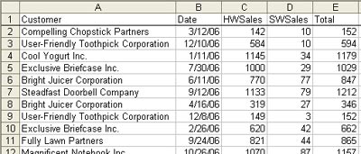 Method 1: SUMIF
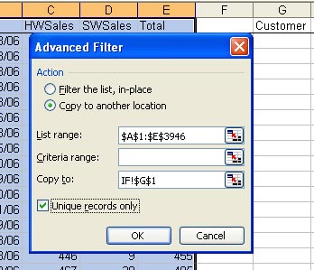 This will give you a unique list of customers in column G.
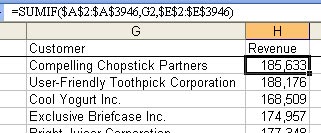 Method 2: Subtotals
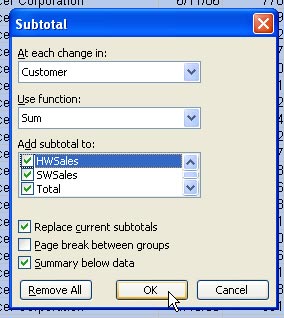 4. Press the "2" group and outline button to show a summary.
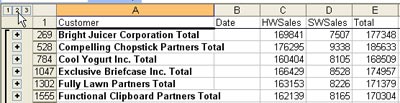 Method 3: Consolidate
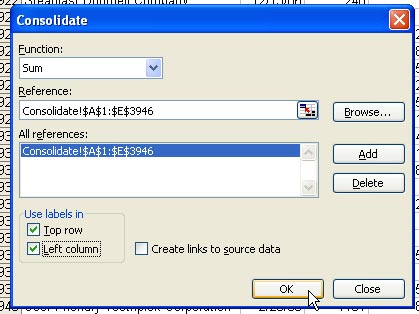 The result: For each unique customer in the left column of your data, you get one row. Excel sums all numeric data, which in this case includes the date field. You will have to delete the date field.
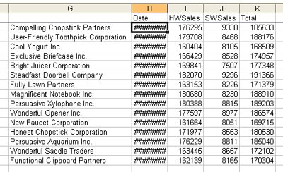 Method 4: Pivot Table
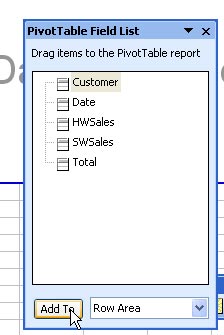 4. Click on Total. Click on Add to Data Area.
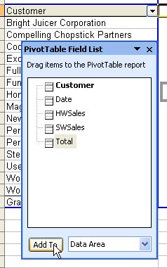 The pivot table is complete.
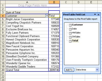


 I made these dropdowns be a different color by using the paint bucket icon in the formatting toolbar. If you click the little dropdown next to the paint bucket, you can access more colors.
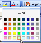 To add the dropdown, select the cell and use Data - Validation. Change the Allow box to be a List. You can then specify where your list is stored.
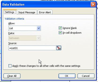 You will see that my list is stored in a place called =List01. This a named range. Most of the time, you could just set up a list off in the far-right unused columns of the spreadsheet. You could say your list is in =AA1:AA2. However, I always have a fear that someone would accidentally delete row 2, wiping out my list. So, I prefer to keep the lists on a hidden Sheet2.If you use Format - Sheet - Unhide, you can Sheet2. There is a fair amount of data stored back here.To find a particular list, use the dropdown to the left of the formula bar. Here is List03.
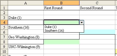
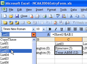 Here is the somewhat interesting thing. How do you make the second round dropdowns work? They seem to be smart enough to know that you selected Duke and UNC Wilmington.
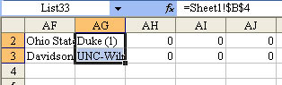
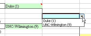 If you look at the Data Validation for this dropdown, you will see that it is defined as List33.Find List33 in the Name dropdown. You will see that it is cells AG2 & AG3 on Sheet2. When you look at these cells, they are formulas that point back to cell B4 and B8 on Sheet1. This is kind of cool - you set up validation to point to a range on the worksheet and that range contains formulas. As long as you don't try to use the dropdown in Round 2 before selecting the winners in Round 1, everything works fine.