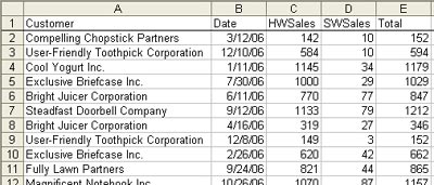
 Method 1: SUMIF
1. Copy the Customer heading to a blank cell G1.
2. From the menu, Data - Filter - Advanced Filter.
3. In the Advanced Filter dialog, choose Copy to New Location, Unique Values. Specify G1 as the output range
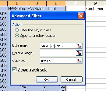 This will give you a unique list of customers in column G.
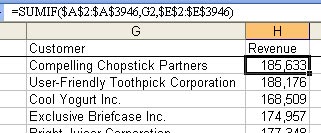
4. The formula in H2 is =SUMIF($A$2:$A$3946,G2,$E$2:$E$3946) 5. Copy the formula down to the other rows in column H. Results:
 Method 2: Subtotals
1. Choose a single cell in column A.
2. Click the AZ sort button in the standard toolbar.
3. From the menu, select Data - Subtotals. Fill out the dialog like this:
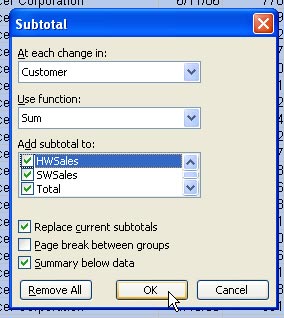 4. Press the "2" group and outline button to show a summary.
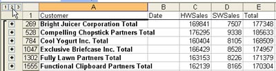 Method 3: Consolidate
1. Select a blank cell to the right of your data.
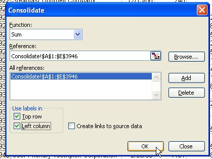
2. From the menu, Data - Consolidate.
3. Fill out the Consolidate dialog as follows:
 The result: For each unique customer in the left column of your data, you get one row. Excel sums all numeric data, which in this case includes the date field. You will have to delete the date field.
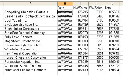 Method 4: Pivot Table
1. Select a single cell in your data. From the menu, Data - Pivot Table and PivotChart Report.
2. Click Finish.
3. Click on Customer. Click Add to Row Area.
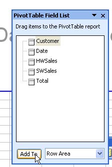 4. Click on Total. Click on Add to Data Area.
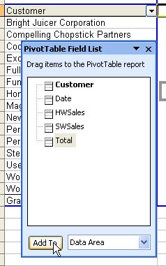 The pivot table is complete.
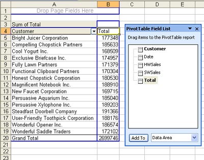
No comments:
Post a Comment