Setting up Data Validation Lists in Excel

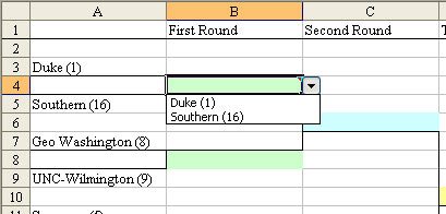
his is the first in a series of articles about the Excel techniques behind my March Madness worksheets. Today, a quick look at the Entry form and how to set up dropdowns in Excel.

In the bracket worksheet, there are dropdowns in all of the cells where you need to select a winner.

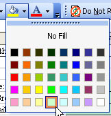
I made these dropdowns be a different color by using the paint bucket icon in the formatting toolbar. If you click the little dropdown next to the paint bucket, you can access more colors.

To add the dropdown, select the cell and use Data - Validation. Change the Allow box to be a List. You can then specify where your list is stored.

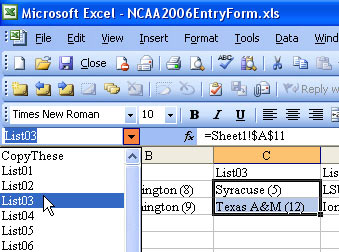
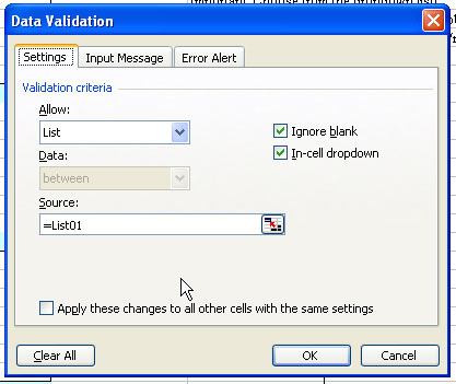You will see that my list is stored in a place called =List01. This a named range. Most of the time, you could just set up a list off in the far-right unused columns of the spreadsheet. You could say your list is in =AA1:AA2. However, I always have a fear that someone would accidentally delete row 2, wiping out my list. So, I prefer to keep the lists on a hidden Sheet2.

If you use Format - Sheet - Unhide, you can Sheet2. There is a fair amount of data stored back here.

To find a particular list, use the dropdown to the left of the formula bar. Here is List03.

Here is the somewhat interesting thing. How do you make the second round dropdowns work? They seem to be smart enough to know that you selected Duke and UNC Wilmington.

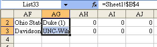
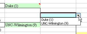If you look at the Data Validation for this dropdown, you will see that it is defined as List33.

Find List33 in the Name dropdown. You will see that it is cells AG2 & AG3 on Sheet2. When you look at these cells, they are formulas that point back to cell B4 and B8 on Sheet1. This is kind of cool - you set up validation to point to a range on the worksheet and that range contains formulas. As long as you don't try to use the dropdown in Round 2 before selecting the winners in Round 1, everything works fine.