Processing Market Research Data in Excel

The tip in this show is from Excel for Marketing Managers.

This new book - Excel for Marketing Managers is one in a new series of books:

• Excel for Scientists and Engineers
• Excel for Teachers
• Excel for Marketing Managers

If you have an idea for another book in this series, drop me a note at consult @ mrexcel.com with your ideas! In today's show, you have hypothetical survey data from surveymonkey.com or some other service. If you look at the data in notepad, it looks like this.

This type of data is comma-delimited. Whenever you have a text file, look at it in notepad first. The other kind of data is space-delimited. When you look at that data in notepad, you will see something that looks like this:

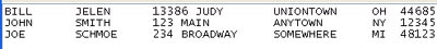Importing to Excel
You can open this data in Excel. Use File - Open. In the Files of Type dropdown, select either All Files or Text Files.

Once you have switched to show text files, click survey.txt and choose Open.

If your file has a .CSV extension, Excel will open it immediately. Otherwise, you go to the Text Import Wizard - step 1 of 3. In this step, you have to choose if your file is delimited or Fixed Width. In this case, survey.txt is delimited, so choose Delimite and click Next.

In step 2, Excel assumes your data is tab-delimited. You will have to choose this checkbox to indicate commas separate each field.

Once you've checked that box, the data preview shows your data in columns.

Click Next to go to Step 3.

If you have date fields, choose the General heading above that field, and indicate the proper date format. My other favorite setting here is the Do Not Import (Skip) setting. If the survey company gave me extra fields that I won't need, I choose to skip them.

Click Finish. Your data will be imported to Excel.

Caution: For the rest of this Excel session, if you try to paste comma-delimited data to Excel, the paste operation will automatically break the data into multiple columns. This is great if you are expecting it, but maddening if you have no idea why it happens somedays and not other days. It is the act of using the Text to Columns Wizard delimited option that causes this "feature" to get turned on. It lasts until the end of the Excel session.

Random Sampling Your manager asks you to randomly call 10% of the survey respondents. Rather than selecting the first 10, enter this formula to the right of your data: =RAND()<=10%. Since RAND() returns a number from 0 to 0.99999, this will mark about 10% of the records with TRUE.

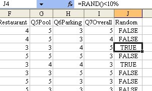Average Response Using Formulas
Go to the first blank row below your data. You would like to average the response. There is an AutoSum icon in the standard toolbar. It is a Greek letter Sigma. Next to this icon is a dropdown arrow. The dropdown arrow contains an option to Average. If you first select all of the columns from C647 to I647, and then choose Average from the dropdown, Excel will add all of the formulas with a single click.

Analyzing Data with a Pivot Table
Say that you want to check front desk ratings over time. Follow these steps.

• Choose a single cell in your data
• From the menu, select Data - Pivot Table and Pivot Chart Report
• Click Next twice.
• In Step 3, click the Layout button.
• Drag Date to the Row area. Drag Q1FrontDesk to the Column Area. Drag Respondents to the Data Area.
• Double click Sum of Respondents in the Data area. Change from Sum to Count.
  

• Click OK. Click Finish.