In episode 166 of the Learn Excel from MrExcel podcast, I talked about using the RandBetween function to create a pair of dice in Excel. I quipped that if you wanted to play Monopoly but were missing the dice, this trick would come in handy. The podcast was an improvement on the technique discussed on page 170 of the book Learn Excel from MrExcel.There is always a better way of doing something in Excel. I received a nice note from viewer Peter Marcaurelle a few days later. He offered up a worksheet that actually had dice that looked liked dice. I've taken Peter's formatting idea and adapted it with my formula. For this week's tip of the week, I would like to present probably the world's longest discussion of creating a pair of dice in Excel.Discussion of RAND vs RANDBETWEEN
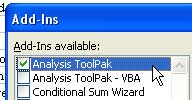
For ten years, I would always build complex formulas using the RAND() function. This function will return a pseudo-random decimal between 0 and 0.999999. To generate a random integer between 0 and 1, you need to wrap the RAND function in a formula like this =INT(RAND()*6)+1. This formula is a little confusing. Multiplying RAND()*6 will generate a number between 0 and 5.999999. Taking the integer portion of that result will return one of these values: 0, 1, 2, 3, 4, or 5. Adding 1 to the result will generate a random integer between 1 and 6. If you are used to using RAND(), you probably can build this formula in your sleep.However, in the analysis toolpack, there is a function called RandBetween. If you want an integer between 1 and 6, simply use =RANDBETWEEN(1,6). This function is a lot easier to remember and since I wrote the book, I've come to prefer RANDBETWEEN to RAND. The one gotcha is that you have to make sure that you have the Analysis Toolpack enabled. Go to Tools - Add-Ins. From the dialog, make sure Analysis Toolpack is checked.
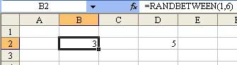
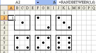
 Once that is installed, then you can create a couple of horrible looking dice using this formula. In the podcast, I started with a couple of cells, each with the =RANDBETWEEN(1,6) formula. Every time you type the F9 key Excel would produce a new set of dice results. Cells B2 and D2 have the same formula to create two dice.
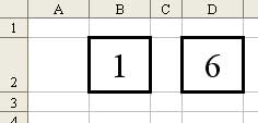
 In the podcast, I suggested using a large centered font with a thick border to make something that looks a bit more like dice.
 Peter realized that if he used Character #108 in the WingDings font, it made a nice dot just like you would see on a die. (I believe the term for the dot on a die is a "pip").
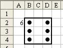
 To use Peter's formatting, I moved the RANDBETWEEN(1,6) formula outside of the dice. For right now, I've put it in cell A2. We will hide it with a white font later, but for right now, let's let it show.
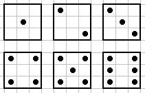
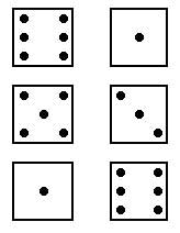
 Here comes the part where we have to think a little bit and study the image of the dice above. There are 9 cells inside of each die. For the top left cell, it should show a dot if the value is equal to 2, 3, 4, 5, or 6. Thus, the formula in cell B2 is =IF(A2>1,CHAR(108),"").The 2nd cell in the top row is never turned on, so there is no formula in C2.The top right cell is turned on for digits 4, 5, and 6. The formula for D2 is =IF(A2>3,CHAR(108),"").In the 2nd row, the left-most column is turned on only for a 6. The formula for B3 is =IF(A2=6,CHAR(108),"")In the 2nd row, the center cell is turned on for 1, 3, or 5. The formula for C3 is =IF(ISODD(A2),CHAR(108),"")The right column of the middle row is turned on only for a 6. The formula for D3 is the same as B3: =IF(A2=6,CHAR(108),"")The bottom right cell is turned on only for 4, 5, and 6. Cell B4 is =IF(A2>3,CHAR(108),"")Cell C4 is never on, so no formula.Cell D4 is on for anything other than a 1, so the formula is the same as B2: =IF(A2>1,CHAR(108),"")You now have a RandBetween function in A2 and a nice representation of the die in B2:D4.
 If you know me, you know that I LOVE to use dollar signs in my cell references so that I can easily copy formulas from one cell to another. However, in this case, I used no dollar signs when referring to cell A2, because I knew that I would later be copying A2:D4 to create additional dice. Here, I've copied that range five additional times to create a total of six dice.
 Every time that you type the F9 key, you will get six new dice values.
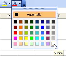
 The final step here is to take the numbers in column A and F and change the font to white. This will in essence hide the numeric values and leave only the dice showing.
 You may also want to use Tools - Options - View and uncheck gridlines to create a cleaner looking worksheet.
For ten years, I would always build complex formulas using the RAND() function. This function will return a pseudo-random decimal between 0 and 0.999999. To generate a random integer between 0 and 1, you need to wrap the RAND function in a formula like this =INT(RAND()*6)+1. This formula is a little confusing. Multiplying RAND()*6 will generate a number between 0 and 5.999999. Taking the integer portion of that result will return one of these values: 0, 1, 2, 3, 4, or 5. Adding 1 to the result will generate a random integer between 1 and 6. If you are used to using RAND(), you probably can build this formula in your sleep.However, in the analysis toolpack, there is a function called RandBetween. If you want an integer between 1 and 6, simply use =RANDBETWEEN(1,6). This function is a lot easier to remember and since I wrote the book, I've come to prefer RANDBETWEEN to RAND. The one gotcha is that you have to make sure that you have the Analysis Toolpack enabled. Go to Tools - Add-Ins. From the dialog, make sure Analysis Toolpack is checked.
Once that is installed, then you can create a couple of horrible looking dice using this formula. In the podcast, I started with a couple of cells, each with the =RANDBETWEEN(1,6) formula. Every time you type the F9 key Excel would produce a new set of dice results. Cells B2 and D2 have the same formula to create two dice.In the podcast, I suggested using a large centered font with a thick border to make something that looks a bit more like dice.Peter realized that if he used Character #108 in the WingDings font, it made a nice dot just like you would see on a die. (I believe the term for the dot on a die is a "pip").- Select several columns. Use Format - Column - Width to set the column width to 2.17.
- Use the thick border tool to draw a border around a 3x3 range of cells.
- Set the font to WingDings
- Keep the font size at 10
- Center the cells.
- Use the formula =CHAR(108) in various cells to create the pips on the die
To use Peter's formatting, I moved the RANDBETWEEN(1,6) formula outside of the dice. For right now, I've put it in cell A2. We will hide it with a white font later, but for right now, let's let it show.Here comes the part where we have to think a little bit and study the image of the dice above. There are 9 cells inside of each die. For the top left cell, it should show a dot if the value is equal to 2, 3, 4, 5, or 6. Thus, the formula in cell B2 is =IF(A2>1,CHAR(108),"").The 2nd cell in the top row is never turned on, so there is no formula in C2.The top right cell is turned on for digits 4, 5, and 6. The formula for D2 is =IF(A2>3,CHAR(108),"").In the 2nd row, the left-most column is turned on only for a 6. The formula for B3 is =IF(A2=6,CHAR(108),"")In the 2nd row, the center cell is turned on for 1, 3, or 5. The formula for C3 is =IF(ISODD(A2),CHAR(108),"")The right column of the middle row is turned on only for a 6. The formula for D3 is the same as B3: =IF(A2=6,CHAR(108),"")The bottom right cell is turned on only for 4, 5, and 6. Cell B4 is =IF(A2>3,CHAR(108),"")Cell C4 is never on, so no formula.Cell D4 is on for anything other than a 1, so the formula is the same as B2: =IF(A2>1,CHAR(108),"")You now have a RandBetween function in A2 and a nice representation of the die in B2:D4.If you know me, you know that I LOVE to use dollar signs in my cell references so that I can easily copy formulas from one cell to another. However, in this case, I used no dollar signs when referring to cell A2, because I knew that I would later be copying A2:D4 to create additional dice. Here, I've copied that range five additional times to create a total of six dice.Every time that you type the F9 key, you will get six new dice values.The final step here is to take the numbers in column A and F and change the font to white. This will in essence hide the numeric values and leave only the dice showing.You may also want to use Tools - Options - View and uncheck gridlines to create a cleaner looking worksheet.
No comments:
Post a Comment